SVDecon: Detail Recovery through Spatially Variant Distortion Correction

Unique amongst its peers, the GPU-accelerated SVDecon module in StarTools, is robust in the face of severe noise, singularities (such as over-exposing star cores), extreme non-linear processing and local detail enhancement, and variable Point Spread Functions. Left: original at 200% zoom. Right: deconvolved with Spatially Variant PSF Deconvolution at 200% zoom.

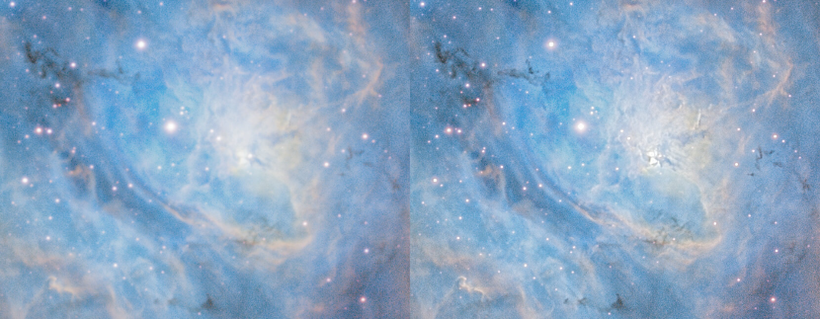
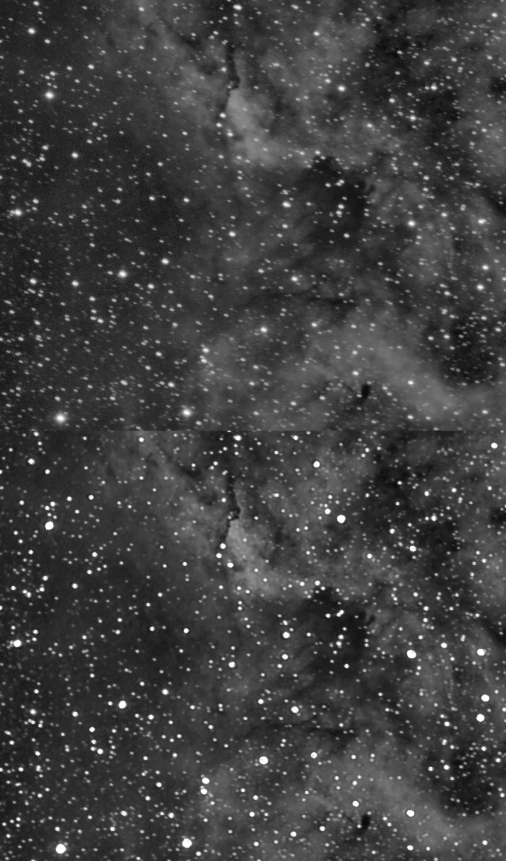
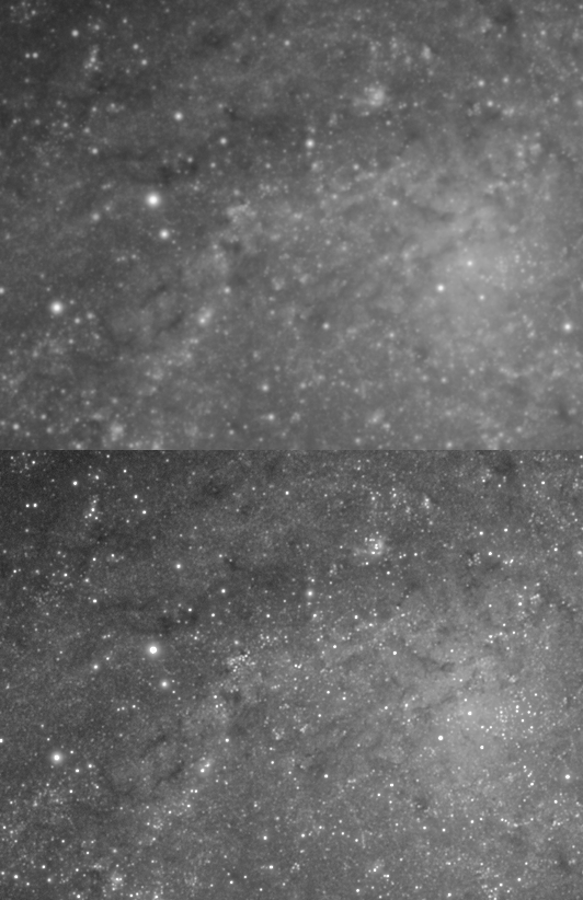
StarTools is the first and only software for astrophotography to implements true, fully generalised Spatially Variant PSF deconvolution (aka "anisotropic" or "adaptive kernel" deconvolution). The fully GPU accelerated solution is robust in the face of even severe noise, meaning it can deployed to restore detail in almost real-time in almost every dataset.

Even the best optical systems will suffer from minute differences in Point Spread Functions (aka "blur functions") across the image. Therefore, a generalised deconvolution solution that can take these changing distortions into account, has been one of the holy grails of astronomical image processing.

Innovations at a glance

The SVDecon module incorporates a series of unique innovations that sets it apart from all other legacy implementations as found in other software;

• It corrects for multiple, different distortions at different locations in the dataset, rather than just one distortion for the entire dataset
  
• It preferably operates on highly processed and stretched data (provided StarTools' signal evolution Tracking is engaged)
• It performs intra-iteration resampling of PSFs
• It is almost always able to provide meaningful improvements, even when dealing with marginal datasets and signals
  
• It is robust in the presence of severe noise, as well as natural singularities (e.g. over-exposed star cores) in the dataset
  
• Depending on your system, previews complete in near-real-time
• Any development of noise grain is tracked and marked for removal/mitigation during final noise reduction
  
• Smart caching allows faster tweaking of some parameters (such as de-ringing) without needing re-doing full deconvolution
• Doing all this, the algorithm at its core, is still based on true Richardson & Lucy deconvolution, and thus its behavior is well understood, documented and accepted in the scientific community, as opposed to black-box neural hallucination-based image re-interpretation algorithms.
  

Usage

Even this heavily distorted dataset with changing trailing direction from corner-to-corner can be improved.

It is important to understand two things about deconvolution as a basic, fundamental process;

• Deconvolution is "an ill-posed problem", due to the presence of noise in every dataset. This means that there is no one perfect solution, but rather a range of approximations to the "perfect" solution.
  
• Deconvolution should not be confused or equated with sharpening; deconvolution should be seen as a means to restore a compromised (distorted by atmospheric turbulence and/or diffraction by the optics) dataset. It is not meant as an acuity enhancing process or some sort of beautification filter. You should (will) always be able to corroborate the detail it restores, using the work from your peers, observatories and space agencies.
  

In addition to the above, deconvolution with a spatially variant Point Spread Function, adds to the complexity of basic deconvolution by requiring a model that accurately describes how the Point Spread Function changes across the image, rather than assuming a one-distortion-fits-all.

Understanding these important points will make clear why some of the various parameters exist in this module, and what is being achieved by the module.

Modes of operation

The SVDecon module can operate in several implicit modes, depending on how many star samples - if any - are provided;

• When no star samples are provided, the SVDecon module will operate in a similar way to the pre-1.7 deconvolution modules.; a selection of synthetic models are available to model one specific atmospheric or optical distortion that is true for the entire image.
• When one star sample is provided, the SVDecon module will operate in a way similar to the 1.7 module (though somewhat more effectively); a single sample provides the atmospheric distortion model for the entire image, while an optional synthetic optics model provides further refinement.
• When multiple star samples are provided, the SVDecon module will operate in the most advanced way. Multiple samples provide a distortion model that varies per location in the image. An optional optical synthetic model may be used for further refinement, though is usually best turned off.

The latter mode of operation is usually the preferred and recommended way of using the module, and takes full advantage of the module's unique spatially variant PSF modelling and correction capabilities.

The module automatically grays out parameters that are not being used, and may also change (zero-out or disable) some parameters in line with the different modes as they are accessed.

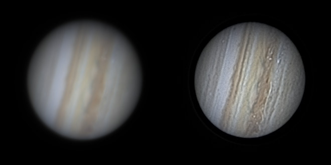
When the subject is lunar or planetary in nature, no star samples are typically available. The "Planetary/Lunar" preset button configures the module for optimal use in these situations.

Finally, details of the mode being used, are reflected in the message below the image window.

Apodization Mask

The SVDecon module requires a mask that marks the boundaries of stellar profiles. Pixels that fall inside the masked areas (designated "green" in the mask editor), are used during local PSF model construction. Pixels that fall outside the masked area are disregarded during local PSF model construction.

It is highly recommended to to include as much of a star's stellar profile in the mask as possible. Failure to do so may lead to increased ringing artifacts around deconvolved stars. Sometimes a simple manual "Grow" operation in the mask editor suffices, in order to include more of the stellar profiles.

Compared to most other deconvolution implementations, the SVDecon module is robust in the face of singularities (for example over-exposing star cores). In fact, it is able to coalesce such singularities further. As such, the mask is no longer primarily used for designating singularities in the image, like it was in versions of StarTools before version 1.8.

The mask does however double as a rough guide for the de-ringing algorithm, indicating areas where of ringing may develop. Clearing the mask (all pixels off/not green in the mask editor) is generally recommended for non-stellar objects, including lunar, planetary or solar data. As a courtesy, this clearing is performed automatically when selecting the Planetary/Lunar preset.

Point Spread Functions (PSFs)

A deconvolution algorithm's task, is to reverse the blur caused by the atmosphere and optics. Stars, for example, are so far away that they should really render as single-pixel point lights. However in most images, stellar profiles of non-overexposing stars show the point light spread out across neighbouring pixels, yielding a brighter core surrounded by light tapering off. Further diffraction may be caused by spider vanes and/or other obstructions in the Optical Tube Array, for example yielding diffraction spikes. Even the mere act of imaging through a circular opening (which is obviously unavoidable) causes diffraction and thus "blurring" of the incoming light.

The point light's energy is scattered/spread around its actual location, yielding the blur. The way a point light is blurred like this, is also called a Point Spread Function (PSF). Of course, all light in your image is spread according to a Point Spread Function (PSF), not just the stars. Deconvolution is all about modelling this PSF, then finding and applying its reverse to the best of our abilities.

Introducing Spatial Variance

Traditional deconvolution, as found in all other applications, assumes the Point Spread Function is the same across the image, in order to reduce computational and analytical complexity. However, in real-world applications the Point Spread Function will vary for each (X, Y) location in a dataset. These differences may be large or small, however always noticeable and present; no real-world optical system is perfect. Ergo, in a real-world scenario, a Point Spread Function that perfectly describes the distortion in one area of the dataset, is typically incorrect for another area of that same dataset.

Traditionally, the "solution" to this problem has been to find a single, best-compromise PSF that works "well enough" for the entire image. This is necessarily coupled with reducing the amount of deconvolution possible before artifacts start to appear (due to the PSF not being accurate for all areas in the dataset).

Being able to use a unique PSF for every (X, Y) location in the image solves aforementioned problems, allowing for superior recovery of detail without being limited by artifacts as quickly.

Synthetic vs sampled PSFs

The SVDecon module, makes a distinction between two types of Point Spread Functions; synthetic and sampled Point Spread Functions. Depending on the implicit mode the module operates in, synthetic, sampled, or both synthetic and sampled PSFs are used.

When no samples are provided (for example on first launch of the SVDecon module), the module will fall back on a purely synthetic model for the PSF. As mentioned before, this mode uses the single PSF for the entire image. As such the module is not operating in its spatially variant mode, but rather behaves like a traditional, single-PSF model, deconvolution algorithm as found in all other software. Even in this mode, its results should be superior to most other implementations, thanks to signal evolution Tracking directing artefact suppression.

A number of parameters can be controlled separately for the synthetic and sampled Point Spread Function deconvolution stages.

Synthetic PSFs

Synthetic PSF models

Atmospheric and lens-related blur is easily modelled, as its behaviour and effects on long exposure photography has been well studied over the decades. 5 subtly different models are available for selection via the 'Synthetic PSF Model' parameter;

• 'Gaussian' uses a Gaussian distribution to model atmospheric blurring.
• 'Circle of Confusion' models the way light rays from a lens are unable to come to a perfect focus when imaging a point source (aka the 'Circle of Confusion'). This distribution is suitable for images taken outside of Earth's atmosphere or images where Earth's atmosphere did otherwise not distort the image.
  
• 'Moffat Beta=4.765 (Trujillo)' uses a Moffat distribution with a Beta factor of 4.765. Trujillo et al (2001) propose in their paper that this value (and its resulting PSF) is the best fit for prevailing atmospheric turbulence theory.
  
• 'Moffat Beta=3.0 (Saglia, FALT)' uses Moffat distribution with a Beta factor of 3.0, which is a rough average of the values tested by Saglia et al (1993). The value of ~3.0 also corresponds with the findings Bendinelli et al (1988) and was implemented as the default in the FALT software at ESO, as a result of studying the Mayall II cluster.
• 'Moffat Beta=2.5 (IRAF)' uses a Moffat distribution with a Beta factor of 2.5, as implemented in the IRAF software suite by the United States National Optical Astronomy Observatory.

Only the 'Circle of Confusion' model is available for further refinement when samples are available. This allows the user to further refine the sample-corrected dataset if desired, assuming any remaining error is the result of 'Circle of Confusion' issues (optics-related) with all other issues corrected for as much as possible.

The PSF radius input for the chosen synthetic model, is controlled by the 'Synthetic PSF Radius' parameter. This parameter corresponds to the approximate the area over which the light was spread; reversing a larger 'blur' (for example in a narrow field dataset) will require a larger radius than a smaller 'blur' (for example in a wide field dataset).

The 'Synthetic Iterations' parameter specifies the amount of iterations the deconvolution algorithm will go through, reversing the type of synthetic 'blur' specified by the 'Synthetic PSF Model'. Increasing this parameter will make the effect more pronounced, yielding better results up until a point where noise gradually starts to increase. Find the best trade-off in terms of noise increase (if any) and recovered detail, bearing in mind that StarTools signal evolution Tracking will meticulously track noise propagation and can snuff out a large portion of it during the Denoise stage when you switch Tracking off. A higher number of iterations will make rendering times take longer - you may wish to use a smaller preview in this case.

Sampled PSFs

Sampled PSF models

Ideally, rather than relying on a single synthetic PSF, multiple Point Spread Functions are provided instead, by means of carefully selected samples. These samples should take the form of. isolated stars on an even background that do not over expose, nor are too dim. Ideally, these samples are provided for all areas across the image, so that the module can analyse and model how the PSF changes from pixel-to-pixel for all areas of the image.

Recommended workflow

The SVDecon module is ideally operated by selecting samples of good quality. Top left; 200% zoom original image. Top right; the resulting deconvolved image by selecting the samples indicated. Bottom left; "Sample Quality" view without samples selected. Bottom right; "Sample Quality" view with three good quality samples selected. The blue bounding boxes should ideally fit the entire green "blobs" (signifiying the apodization mask for each sample).

As opposed to all other implementations of deconvolution in other software, the usage of the SVDecon module is generally recommended towards the end of your luminance (detail enhancement) processing workflow. That is, ideally, you will have already carried out the bulk of your stretching and detail enhancement before launching the SVDecon module. The reason for this, is that the SVDecon module makes extensive use of knowledge that indicates how you processed your data prior to invoking it, and how detail evolved and changed during your processing. This knowledge specifically feeds into the way noise and artifacts are detected and suppressed during the regularisation stage for each iteration.

For most datasets, superior results are achieved by using the module in Spatially Variant mode, e.g by providing multiple star samples. In cases where providing star samples is too difficult or time consuming, the default synthetic model will still very good results however.

Selecting samples for Spatially Variant deconvolution

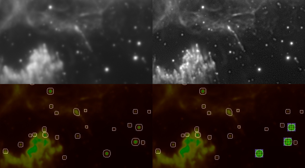
To provide the module with PSF samples, a the 'Sampling' view should be selected. This view is accessed by clicking the 'Sampling' button in the top right corner. This special was designed to help the user identify and select good quality star samples.

In the 'Sampling' view, A convenient rendering of the image is shown, in which;

• Candidate stars are delineated by an outline.
• Red pixels show low quality areas
• Yellow pixels show borderline usable areas.
• Green pixels show high quality areas.
  

Ideally, you should endeavour to find stars samples that have a green inner core without any red pixels at their centre. If you cannot find such stars and you need samples in a specific area you may choose samples that have a yellow core instead. As a rule of thumb, providing samples in all areas of the image takes precedence over the quality of the samples.

You should avoid;

• Stars that sit on top of nebulosity or other detail.
• Objects that are not stars (for example distant galaxies)
  
• Stars that are close to other stars
  
• Stars that appear markedly different in shape compared to other stars nearby
• Stars whose outline appear non-oval or concave or markedly different to the outlines of other stars nearby

Detail should snap into focus, stars should coalesce into point lights and halos around over-exposing stars should be diminished.

Star samples can be made visible on the regular view (e.g. the view with the before/after deconvolved result) by holding the left mouse button. Star samples will also be visible outside any preview area, this also doubles as a reminder that any selected PSF Resampling algorithm will not resample those stars (see 'PSF resampling mode'). You may also quickly de-select stars via the regular before/after view by clicking on a star that has a sample over it that you wish to remove.

The Sampled Area

The immediate area of a sampled star is indicated by a blue square ('bounding box'). This area is the 'Sampled Area'. A sampled area should contain one star sample only; you should avoid selecting samples that have parts of other stars in the blue square surrounding a prospective sample. The size of the blue square is determined by the 'Sampled Area' parameter. The 'Sampled Area' parameter should be set in such a way that all samples' green pixels fall well within the blue area's confines and are not 'cut-off' by the blue square's boundaries.

Star sample outlines and apodization mask

The star sample outlines are constructed using the apodization mask that is generated. You may touch up this mask to avoid low-quality stars being included in the blue square 'Sampled Area', if that helps to better sample a high quality star.

Number of samples and location of samples

Ideally samples are specified in all areas of the image in equal numbers. The module will work with any amount of samples, however ten or more, good quality samples is recommended. The amount of samples you should provide is largely dependent on how severe the distortions are in the image and how they vary across the image.

Please note that, when clicking a sample, the indicated centre of a sample will not necessarily be the pixel you clicked, nor necessarily the brightest pixel. Instead, the indicated centre is the "luminance centroid". It is the weighted (by brightness) mean of all pixels in the sample. This is so that, for example, samples of stars that are deformed or heavily defocused (where their centre is less bright than their surroundings) are still captured correctly.

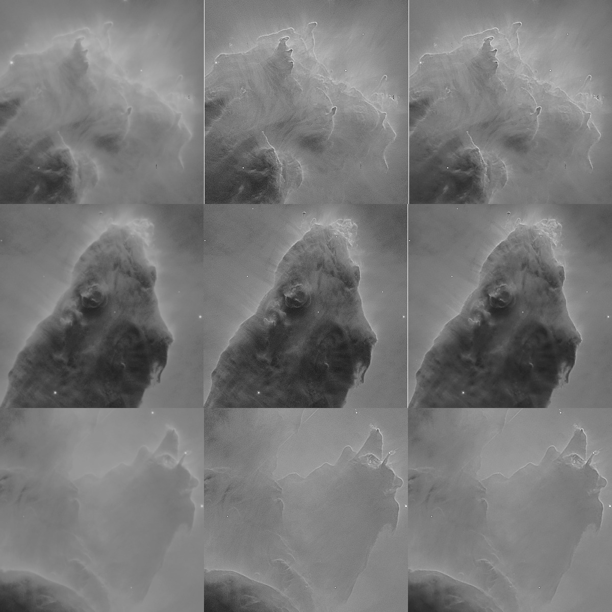
Heavily distorted PSFs

For images with heavily distorted PSFs that are highly variant (for example due to field rotation, tracking error, field curvature, coma, camera mounting issue, or some other acquisition issue that has severely deformed stars in an anisotropic way), the 'Spatial Error' parameter may need to be increased, with the 'Sampled Iterations' increased in tandem. The 'Spatial Error' parameter relaxes locality constraints on the recovered detail, and increasing this parameter, allows the algorithm to reconstruct point lights from pixels that are much less co-located than would normally be the case. Deconvolution is not a 100% cure for such issues, and its corrective effect is limited by what the data can bear without artifacts (due to noise) becoming a limiting factor.

Under such challenging conditions, improvement should be regarded in the context of improved detail, rather than perfectly point or circle-like stellar profiles. While stars may definitely become more pin-point and/or 'rounder', particularly areas that are (or are close to) over-exposing, such as very bright stars, may not contain enough data for reconstruction due to clipping or non-linearity issues. Binning the resulting image slightly afterwards, may somewhat help hide issues in the stellar profiles. Alternatively, the Repair module may help correcting these stars.

Just using synthetic PSF modelling, the SVDecon module is just as effective on lunar, planetary and solar datasets, as it is on deep space datasets.

PSF Resampling mode

The SVDecon module is innovative in many ways, and one such innovation is its ability to re-sample the stars as they are being deconvolved. This feedback tends to reduce the development of ringing artifacts and can improve results further.

Three 'PSF Resampling' modes are available;

• None; no resampling and model reconstruction occurs during deconvolution - the samples are used as-is.
  
• Intra-Iteration; all samples are resampled at their original locations for each iteration
  
• Intra-Iteration + Centroid Tracking; all samples are resampled after their locations have first been re-determined.Intra-iteration resampling while a preview is being used will only re-sample the samples that are contained within the preview. Therefore, the full effects of intra-iteration resampling are best evaluated without a preview being defined. As, depending on your system's CPU and GPU resources, intra-iteration resampling may be rather taxing, it may be useful to evaluate its effects only once all samples are set and once you are happy with the results without PSF resampling activated.
  

Dynamic Range Extension

The 'Dynamic Range Extension' parameter provides any reconstructed highlights with 'room' to show their detail, rather than clipping themt against the white point of the input image. Use this parameter if significant latent detail is recovered that requires more dynamic range to be fully appreciated. Lunar datasets can often benefit from an extended dynamic range allocation.

Planetary, solar and lunar datasets

A preset for lunar, planetary, solar use quickly configures the module for lunar, planetary and solar purposes; it clears the apodization mask (no star sampling possible/needed) and dials in a much higher amount of iterations. It also dials in a large synthetic PSF radius more suitable to reverse atmospheric turbulence-induced blur for high magnification datasets. You will likely want to increase the amount of iterations further, as well as adjust the PSF radius to better model the specific seeing conditions.

Evaluating the result

A considerable amount of research and development has gone into CPU and GPU optimisation of the algorithm; an important part of image processing is getting accurate feedback as soon as possible on decisions made, samples set, and parameters tweaked.

As a result, it is possible to evaluate the result of including and excluding samples in near-real-time; you do not need to wait minutes for the algorithm to complete. This is particularly the case when a smaller preview area is selected.

As stated previously, please note however, that the 'PSF Resampling' feature is only carried out on any samples that exist in the preview area. As a result, when a 'PSF Resampling' mode is selected, previews may differ somewhat from the full image. To achieve a preview for an area when a 'PSF Resampling' mode is selected, try to include as many samples in the preview area as possible when defining the preview area's bounding box.

With the aforementioned caveat with regards to resampling in mind however, any samples that fall outside the preview are still used for construction of the local PSF models for pixels inside the preview. In other words, the results in the preview should be near-identical to deconvolution of the full image, unless a specific 'PSF Resampling' mode is used.

SVDecon can greatly improve the clarity of image data from even space telescopes and probes such as the Hubble Space Telescope. Left column: original data, Center column: SV deconvolved data, Right column: default noise mitigation during final signal Tracking Denoise stage, demonstrating precise, autonomous deconvolution-induced grain and artifact tracking.

Noise and artifact propagation

While it is best to avoid overly aggressive settings that exacerbate noise grain (for example by specifying a too large number of iterations), a significant portion of such grain will be still be very effectively addressed during the final noise reduction stage; StarTools' Tracking engine will have pin-pointed the noise grain and its severity and should be able to significantly reduce its prevalence during final noise reduction (e.g. when switching Tracking off).

Ringing artifacts and/or singularity-related artifacts are harder to address and their development are best avoided in the first place by choosing appropriate settings. As a last resort, the 'Deringing Amount', 'Deringing Detect' and 'Deringing Fuzz' parameters can be used to help mitigate their prevalence.

Recovering PSF samples from the log

Any samples you set, are stored in the StarTools.log file and can be restored using the 'LoadPSFs' button.

In the StarTools.log file, you should find entries like these;

PSF samples used (8 PSF sample locations, BASE64 encoded)

VFMAAAgAOAQMA/oDEQHaAoEAIwNeAOQAUwDUAY8AbAI5AdMBMQGkAFAB

If you wish to restore the samples used, put the BASE64 string (starting with VFM... in the example) in a text file. Simply load the the file using the 'LoadPSFs' button.